I turned a boring task list into a mini Excel app in 10 minutes

Lots of task-tracking software is costly and comes with more features than you need. I built a dynamic task tracker that does everything I need in three quick steps—and if you have Excel for Microsoft 365 or Excel for the web and a spare 10 minutes, you can too.

Step 1: Build your basic list

Start with two columns

Open a blank worksheet and set the font for all cells to 16pt. Then, starting in D4, create two columns called Task Name and Status, and adjust the Task Name column width so there’s plenty of room to write your tasks.

Start with 10 ordinary tasks. You can replace them with real tasks later on:

• Book dentist appointment
• Pay electricity bill
• Buy groceries
• Reply to important emails
• Clean out the fridge
• Back up computer files
• Return unwanted purchase
• Book car service
• Renew insurance
• Plan meals for next week

Select the two columns and press Ctrl+T to turn them into an Excel table. When Excel asks whether your table has headers, make sure that box is checked.

With the table still selected, in the Table Design tab, uncheck Banded Rows and Filter Button. This gives your table a cleaner look without unnecessary visual distractions. Also, change the table name on the left side of the same tab to T_Tasks, then press Enter.

Finally, select the Status column, open the Insert tab, and click Checkbox. You’ll now be able to check a box beside each task when you’ve finished it.

That’s the basic setup done. Now you can make Excel keep track of what you’ve actually accomplished.

Step 2: Add the formulas that make the tracker dynamic

Let Excel keep track of your progress

The key is to use formulas that keep everything up to date as you add and complete tasks.

Before adding the dashboard, though, take a moment to reduce the widths of columns A and C to about 20 pixels. These are simply buffers around the main content and give the layout a little breathing room.

Now, at the top of the dashboard, select cells D2:E2 and, in the Home tab, click Merge & Center. Then, fill the merged cells with light gray, type this formula, and press Enter:

=COUNTIFS(T_Tasks[Status],TRUE)/ROWS(T_Tasks)

Format the result as a Percentage in the Number group on the Home tab.

Next, create the task count area.

In B4, type TOTAL TASKS, and widen the column so the text fits comfortably. Select the Task Name table column header, click the Format Painter button in the Home tab, and click cell B4, the TOTAL TASKS header. Remove the borders from this title cell and center the text.

Then merge cells B5:B6, apply a light gray fill, and enter:

=ROWS(T_Tasks)

Next, it’s the PENDING section. Rather than creating this from scratch, copy the TOTAL TASKS heading and result area, and paste it in cells B8:B10. Then, replace TOTAL TASKS with PENDING, change the heading’s background to red, and swap the existing formula for this one:

=COUNTIFS(T_Tasks[Status],FALSE)

For COMPLETED, copy the whole PENDING area and paste it in cells B12:B14. Change the text to COMPLETED, format the background with a green fill, and change FALSE in the formula to TRUE, so you end up with this:

=COUNTIFS(T_Tasks[Status],TRUE)

Finally, select the four merged areas by holding Ctrl while you click them, and increase the font size to around 26pt. Center them horizontally and vertically in the Home tab so the dashboard starts to look more like a little productivity app and less like a collection of cells.

The useful thing about these formulas is that you don’t have to maintain the dashboard yourself. Add another task to the table, and the total changes. Tick a checkbox, and the pending and completed counts change too.

Step 3: Give your tracker a satisfying finishing touch

Make completed tasks go gray and the progress bar stand out

The tracker already works, but you can give it a little more visual feedback. First, let’s make the tasks turn gray with strikethrough when you complete them.

Select the entire Task Name table column, click Conditional Formatting in the Home tab, and select New Rule. Then, click Use a formula to determine which cells to format, and enter:

=$E5=TRUE

Click Format to set the font color to gray and apply strikethrough.

Now, when you tick a task’s checkbox, its name gets crossed out automatically. It’s a small thing, but it makes the list much easier to scan because you can immediately see which jobs you’ve dealt with.

Next, turn the percentage at the top into a proper progress bar.

Select the merged progress cell and go to Conditional Formatting > Data Bars > More Rules. Set the minimum to Number — 0 and the maximum to Number — 1. Choose a green fill and select No Border. Because the underlying formula produces a decimal between 0 and 1, the bar now grows as you complete more tasks.

At this point, test everything rather than assuming you’ve built it correctly. Add a few new rows to the table and make sure the total changes. Tick and untick some checkboxes and watch the pending count, completed count, percentage, strikethrough formatting, and progress bar respond.

If you’ve finished a task and don’t want it cluttering up the list anymore, right-click its table row and choose Delete > Table Rows. The table shrinks and the dashboard formulas update automatically.

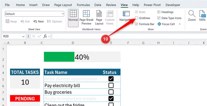
Finally, go to the View tab and uncheck Gridlines. I like doing this last because it’s the little detail that makes the finished tracker feel much more like a simple productivity app than a spreadsheet.

Excel is a pretty good geeky playground

If you have another 10 minutes to spare, why not take your personal organization a step further by building a swanky timeline from a simple line chart? I like projects like this because they remind me that Excel doesn’t always have to be about work. Once you start experimenting with what the grid, formulas, checkboxes, and formatting can do, a blank worksheet becomes a surprisingly good place to spend a spare bit of time.