I turned my giant Excel formula into something I can actually understand

We all know someone who loves building a ridiculously complicated Excel formula and proudly announcing that it works. I used to be that person. I’ve been writing Excel formulas for decades, and I loved the satisfaction of making a single formula handle a problem that once seemed impossible. The trouble was, those formulas could become a lot less impressive when I came back to them later. Then along came the LET function.

My long Excel formula worked fine—until I had to read it

It felt like cracking the Enigma code

Take this Excel table as an example. It contains nine columns, four of which feed into the performance score out of 100 for whichever salesperson I select in cell B1. The score combines three measures: 50 points for how much of their sales target they’ve achieved, 30 points for their profit margin, and 20 points for their average customer rating.

Here’s the formula I’d enter into cell B2:

=MIN(SUMIFS(tblSales[Revenue], tblSales[Salesperson], B1)/MAXIFS(tblSales[Sales Target], tblSales[Salesperson], B1), 1)*50+(SUMIFS(tblSales[Profit], tblSales[Salesperson], B1)/SUMIFS(tblSales[Revenue], tblSales[Salesperson], B1))*30+(AVERAGEIFS(tblSales[Customer Rating], tblSales[Salesperson], B1)/5)*20

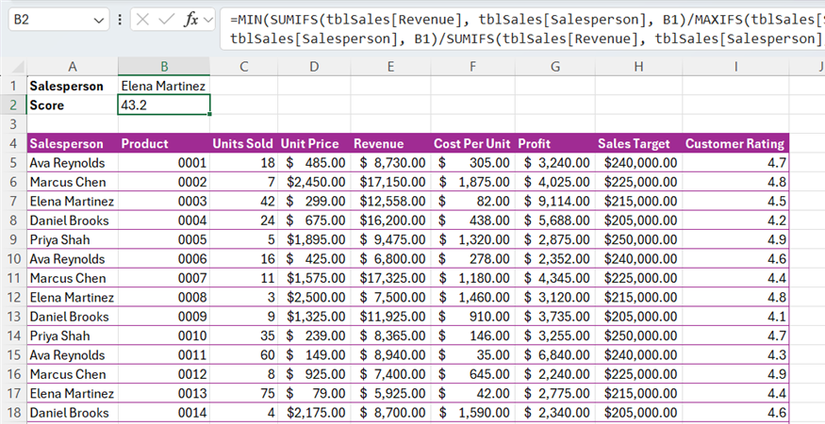
There’s nothing actually wrong with this formula. Excel understands it perfectly well, and it returns the score I expect. The problem is that if I need to change part of it, explain it to someone else, or come back to it a year later, it can take longer to pick apart than it took to build in the first place. I need to spot that one SUMIFS calculates revenue, that MAXIFS retrieves the sales target, that another SUMIFS calculates profit, and that AVERAGEIFS produces the customer rating.

There’s also some repetition hiding in there. I’m calculating total revenue twice: once to work out how much of the target the salesperson has achieved, and again to calculate their profit margin. This makes the formula longer and gives me another piece of logic to maintain if I ever need to change it.

What I really want to see when I look at the formula is the logic behind it: revenue, target, profit, rating, target score, profit margin, and rating score. I don’t want to have to translate a wall of functions, references, and parentheses into those concepts every time I return to the formula.

LET lets me give each calculation a name

The formula suddenly starts talking my language

This is where the LET function—available in Excel for Microsoft 365, Excel 2024 and 2021, and Excel for the web—comes in. I can give each intermediate result a meaningful name, then use those names later in the formula.

First, I’ll tell Excel that I want to use the name revenue for my first calculation. The name comes first, followed by a comma, then the calculation that produces its value:

=LET(
revenue, SUMIFS(tblSales[Revenue], tblSales[Salesperson], B1),

Next, I’ll add the salesperson’s target:

=LET(
revenue, SUMIFS(tblSales[Revenue], tblSales[Salesperson], B1),
target, MAXIFS(tblSales[Sales Target], tblSales[Salesperson], B1),

I’ll do the same thing for profit and the average customer rating:

=LET(
revenue, SUMIFS(tblSales[Revenue], tblSales[Salesperson], B1),
target, MAXIFS(tblSales[Sales Target], tblSales[Salesperson], B1), 
profit, SUMIFS(tblSales[Profit], tblSales[Salesperson], B1), 
rating, AVERAGEIFS(tblSales[Customer Rating], tblSales[Salesperson], B1),

At this point, I’ve replaced four chunks of complicated-looking calculations with four names that tell me exactly what each result represents. More importantly, I can now use those names to build the next part of the calculation.

The targetScore is the salesperson’s revenue divided by their target, capped at 100%. The profitMargin is profit divided by revenue, and the ratingScore is the rating converted from a five-point scale:

=LET(
revenue, SUMIFS(tblSales[Revenue], tblSales[Salesperson], B1),
target, MAXIFS(tblSales[Sales Target], tblSales[Salesperson], B1),
profit, SUMIFS(tblSales[Profit], tblSales[Salesperson], B1),
rating, AVERAGEIFS(tblSales[Customer Rating], tblSales[Salesperson], B1),
targetScore, MIN(revenue/target,1),
profitMargin, profit/revenue,
ratingScore, rating/5,

Finally, I’ll combine those three scores using their respective weightings:

=LET(
revenue, SUMIFS(tblSales[Revenue], tblSales[Salesperson], B1),
target, MAXIFS(tblSales[Sales Target], tblSales[Salesperson], B1),
profit, SUMIFS(tblSales[Profit], tblSales[Salesperson], B1),
rating, AVERAGEIFS(tblSales[Customer Rating], tblSales[Salesperson], B1),
targetScore, MIN(revenue/target,1),
profitMargin, profit/revenue,
ratingScore, rating/5,
(targetScore*50)+(profitMargin*30)+(ratingScore*20)
)

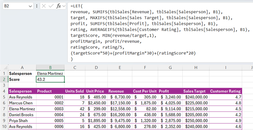
The underlying calculations haven’t changed. I’m still using SUMIFS to calculate revenue and profit, MAXIFS to retrieve the salesperson’s sales target, and AVERAGEIFS to calculate the average customer rating. I’ve simply named those results to reflect what they mean: revenue, target, profit, and rating. These named variables are now clearly listed in the formula, so I can quickly scan them and see the building blocks of the calculation at a glance. I can then use those names to create targetScore, profitMargin, and ratingScore before combining them into the final score calculation.

Also, revenue is now calculated only once and then reused in both targetScore and profitMargin. And if I decide to change one of those calculations or its weighting later, I can find the relevant named component much more easily than I could in the original formula.

This is the part of LET that appeals to me most. I’m still asking Excel to do the same work, but the formula is easier to understand, and the logic is more visible.

Where do helper formulas fit into the equation?

It depends on the intermediate calculations

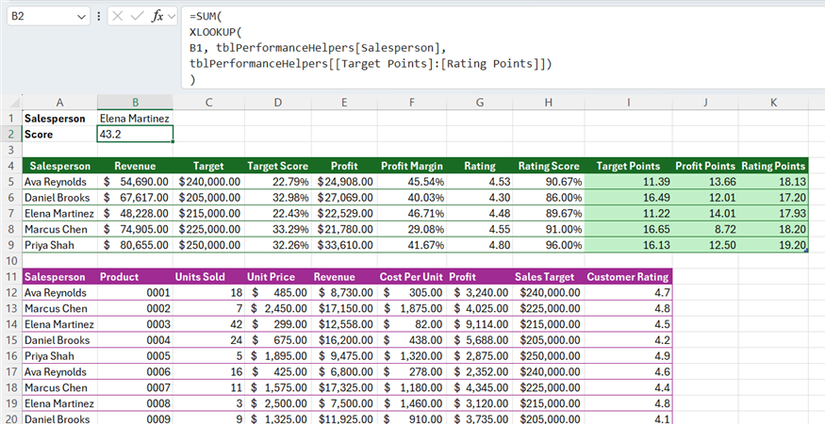
I’m a big fan of helper formulas, whether they’re added as columns to an existing dataset or gathered together in a separate table. The screenshot above shows the trade-off. The helper table makes every intermediate calculation easy to see and reuse, but it also adds a sizable chunk of spreadsheet structure for a calculation that ultimately produces a single value.

I’d choose helper formulas over LET if I wanted to use those intermediate calculations elsewhere, such as in a separate analysis, a chart, or a PivotTable. But the trade-off is that they add extra machinery. Every additional calculation creates another moving part in the workbook, and the more moving parts you have, the more opportunities there are for errors.

So when deciding whether to use LET or helper formulas, I generally follow this rule of thumb: if an intermediate calculation is useful on its own, give it a helper formula. If it’s simply supporting one final result, LET can keep it contained in a single formula while keeping the logic clear.

Yes, I could hide or group the helper calculations, but that adds another layer of spreadsheet structure to navigate and maintain. With LET, I can keep the supporting calculations inside the formula, leave the existing structure intact, and present the final result without adding calculations that most people will never need to see.

My formulas don’t have to be a mystery anymore

Thanks to functions like LET, I no longer have to create long, unreadable formulas that only make sense to me at the time. I can still make Excel do complicated things, but I can also make the logic behind those calculations much easier to understand. And if I want to add even more context, I can tuck in plain-language notes using the N() function trick.